2.1 Introduction
The program for power flow solution using Newton-Raphson method has already developed by Prof. Hadi Saadat of Milwauke University, USA in MATLAB [2]. MATLAB is an interpreted language for numerical computation. MATLAB allows its users to solve problems, produce graphics easily and produce code. The MATLAB code is easy to debug [8].
The MATLAB program is simple to use but lacks of many features in commercial power flow program. These MATLAB program is a stand alone program, therefore it need to be install before user can use it. Because MATLAB is an interpreted language, it can be slow, and poor programming practices can make it acceptably slow [9, 10].
2.2 Load flow analysis
Load flow solution is a solution of the network under steady state condition subjected to certain inequality constraints under which the system operates. These constraints can be in the form of load magnitude, bus voltages, reactive power generation of the generators, tap settings of a tap-changing transformer etc. The load flow solution gives the bus voltages and phase angles, hence the power injection at all the buses and power flow through interconnecting transmission lines can be easily calculated. Load flow solution is essential for designing a new power system as well as for planning an extension or operation of the existing one for varying demand. These analyses require number of load flow solutions under both normal and abnormal (outage of transmission line or outage of some generators) operating conditions. Load flow solution also gives the initial state of the system when the transient behavior of the system is to be studied. Under steady state condition, the network equations will be in the form of simple algebraic equations.
2.2.1 Bus Classification
In a power system each bus or node is associated with four quantities, real and reactive powers, bus voltage magnitudes and its phase angles. In a load flow solution two out of four quantities are specified and the remaining two are to be calculated through the solution of the equations. The buses are classified into the following three types depending upon the quantities specified.
1 Load bus: At this bus the real and reactive components of power are specified. It is desired to find out the voltage magnitude V and phase angle δ through the load flow solution. Voltage at load bus can be allowed to vary within a prescribed value.
2 Generator bus or voltage-controlled bus: Here the voltage magnitude corresponding to the generator voltage V and real power PG corresponding to its ratings is specified. It is required to find out the reactive power generation QG and the phase angle δ of the bus.
3 Slack/Swing or reference bus: Here the voltage magnitude V and phase angle δ is specified. This will take care of the additional power generation required and Transmission losses. It is required to find the real and reactive power generations (PG, QG) at this bus.
2.3 Newton-Raphson load flow (NRLF) Method
2.3.1 Calculation of Jacobian
For an N-bus power system there will be n equations for real power injection P i and n-equations for reactive power injection Q i .

For load buses, voltage magnitudes and phase angle are set to 1.0 and 0.0 respectively.
For voltage-regulated buses phase angle are set to 0.0.
The number of equations to be solved depends upon the specifications we have. If the total number of buses is N;
N = number of PV bus – [2 x number of PQ bus]
Unknowns to be calculated are power angles (δ) at all the buses except slack and bus voltages (V) at load bus. The following method known as Newton- Raphson method is used for solving the unknown quantities. The problem formulation is as follows:

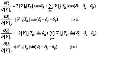
The elements of the Jacobian matrix can be calculated using the following equations

Procedure for this iterative method is for the given system first the Y-bus matrix has to be formed.
Y = G + j B
Where
Y is a bus admittance matrix
G is real part of Y-bus matrix
B is imaginary part of Y-bus matrix
The resistance and reactance of each line have been given for any system from which the admittance matrix can be formed.
Inverse the Jacobian matrix and from matrix equation solve for DVik and D d ik
The new voltage magnitude and phase angles are computed from


k = current iteration
k+1 = next iteration
The calculation process for Vi k+1 and di k+1 stop when the DPik, DQik, DVik and D d ik are very small.
The process is continued until the residuals DPik and DQik are less than the specified accuracy i.e,
k+1 = next iteration
The calculation process for Vi k+1 and di k+1 stop when the DPik, DQik, DVik and D d ik are very small.
The process is continued until the residuals DPik and DQik are less than the specified accuracy i.e,


No comments:
Post a Comment